Li Mineralogy by Automated SEMs: A case study

  Similar to other analytical methods, Automated SEMs have their own restrictions; one of the limitation of SEMs -more specific EDS Spectra analysis-  is that light elements such as Li or Be cannot be detected with the current X-Ray detectors (e.g. Reed 2005). This can effect the reliability of the mineral list or SIP file when dealing with one of these elements, such as Li exploration projects; however an integration with XRD and a  supplementary method such as Laser Ablation ICPMS, enables QEMSCAN or MLA to overcome this technical restriction.

In this post, we are going to review a case study on a Li mineralogy, from a prelim exploration project on Pegmatites with the main objective to identify and characterize main carrier of Li. The mineralogical study was done on 97 core samples with Li abundance of 0.07-0.15 % and 0.05-0.1% of W with the host rock being identified as Alkaline Feldspar Granite; here we will review the results for one sample.

The mineralogy test was initiated using QEMSCAN on one size fraction; the samples were stage pulverised to 125 µ for preparing 30 mm round polished sections; two sections per sample was prepared (one transverse and one normal). BMA measurement mode was used for Modal Mineralogy analysis and PMA mode for particle data. In order to validate the reliability of the SIP file, 25 samples with highest amounts of W and Li  were selected for Q-XRD analysis.

In granites and other similar rocks, the main carrier of Li minerals are silicates, like Pyroxenes ( e.g. Spodumene LiAl(Si₂O₆)), Micas.( e.g. Lepidolite  KLi₂AlSi₄O₁₀F(OH)) or Feldspathoid  ( Petalite LiAlSi₄O₁₀); now regarding the inability of detecting Li by EDS spectra technique, the identification of these minerals can be tricky with probability of misclassification with other minerals or entries; Although elemental ratio (e.g. Si/Al) in the SIP entries can help -to some extend- to avoid such, however an ideal condition - of the sample, measurement settings, sample prep etc- is prerequisite for such discrimination.

After QEMSCAN test and comparison with XRD, it was concluded that the Li minerals in this sample are from Mica group, i.e. Zinnwaldite  (KLiFeAl₂Si₃O₁₀(F_,OH)₂) and Lepidolite KLi₂AlSi₄O₁₀F(OH), with approximate abundance of 2.8% and 1.13%, respectively. Without the XRD check prior to generate the SIP file, the chances of misclassification of K-Feldspar and Lepidolite could occur caused by  overlapping X-Ray counts for Si, Al and K (see the synthesized spectra).

                       Modal Mineralogy wt% by QEMSCAN

Using QEMSCAN SIP editor it is easier to overcome such misclassifications comparing to MLA, where mainly peak shapes match criteria is used for minerals identifications. In addition to elemental counts, as well as Si/Al and K/Al ratio, we also used “May Have” criteria in the SIP entries for both Orthoclase and Lepidolite.

Synthesized EDS spectra by SIP Editor

Li by chemical assay in this sample had resulted 1385 ppm , while calculated Li by QEMSCAN using empirical formula of Lepidolite and Zinnwaldite is ~ 0.11 %. This deficiency for Li is opposite of what was seen for other elements such as K, Si and Al, where they showed a tight reconciliation. So the possibility of underestimation of minerals’ quantification was ruled out. This can be explained by the presence of Li as a minor element in other minerals; looking back at the mineral list, the best candidates are Muscovite and/or Biotites. In order to confirm this, yet another method should be used. For this purpose Laser Ablation ICP-MS is suitable and we can perform the test directly on the same polished sections that were used for mineralogy test by QEMSCAN.

As a brief summary, the L.A. ICP-MS test confirmed the elevated abundance of Li in muscovite with range of 1000-4300 ppm in the analyzed samples; with the +10 wt% presence of Muscovite, this can definitely be the main reason for the difference of Li between mineralogy test and chemical assay. 

Despite the technical restrictions of MLA and QEMSCAN, they still play an important role in mineralogy projects,  using the right supplementary methods can help to overcome these restrictions.

Hope it was interesting for you!

Matt (Mahdi) Ghobadi

Announcing a new technique for SEM super-resolution mineral analysis

This post talks about a newly available technique for analyzing minerals using a scanning electron microscope equipped with EDS detectors, using existing hardware.

The images shown here are an electron back-scatter image, and corresponding mineral map of each pixel in the image analyzed with the new technique.

Figure 1: Automated nanomin analysis of mineral sample (no user intervention)

This approach does not constrain the number of minerals per pixel, unlike a standard QEMSCAN analysis. Rather, it allows multiple minerals to be reported within a single pixel. This goes beyond the EDS limit, revealing sub-pixel detail for the first time. It also allows each mineral to consist of multiple mineral variety end-members that are linked into a solid solution. For example, the plagioclase feldspar solid solution links the albite and anorthite end-member mineral spectra into a solid solution as a single mineral. Any mineral detected on that solid solution is automatically reported as a plagioclase, regardless of the percentage of sodium and calcium in the spectrum. It automatically computes the interchange of sodium and calcium, balancing out the other elements, without any interaction required from the user.

This removes the burden of managing complex mineral chemistry within the analytical software, and frees up time for analysis of the data.

In SEM-EDS mineral analysis, the interaction volume of the EDS signal is approximately 1-5um for typical measurement conditions. That is, each pixel represents the signal from a 5um volume. And when that volume has more than 1 mineral present, the signal measured is a sum of the several minerals, which may or may not have different elements.

The implication here is apparent - any pixel that does not fall wholly within a pure mineral grain should be reported as a mix of minerals. A few commercial SEM-EDS techniques attempt to avoid this problem by trying to avoid measuring pixels that aren’t clearly in the center of a mineral grain. Other try to remediate it by using a statistical approach based on the surrounding mineral classifications to touch-up the classification of the center pixel. Both of these work-arounds will work for a limited set of situations, but they fail where it’s impossible to avoid a fine texture.

Figure 2: Automated QEMSCAN analysis (no user intervention)

The centroid method risks runs a risk that the simplified analysis will miss the important features within the sample. And it also introduces a bias into the result if portions of the sample are skipped or left unclassified. In the image above, an automated QEMSCAN analysis shows large swathes of unclassified pixels, requiring further input from the user. The user must interactively decide whether to skip the unclassified pixels, try to recover them from surrounding data, or manually add mineral entries for the missing minerals. In other words, there is a significant effort required to improve the accuracy from the initial classification. While all these problems can be solved, they also add significant time to the process.

In contrast, the new technique shows a result where the pixels from multiple minerals have been reported, saving a significant amount of time to an operator. The operator has more time for interpreting the results, or classifying other samples.

At the current time, this technique is only offered by FEI (http://www.fei.com) within the Maps-Mineralogy software package.
The only link currently available is https://www.linkedin.com/pulse/finer-side-automated-spatial-mineralogy-lucy-plant

A short history of automated mineralogy colours

The signature output from FEI’s SEM-EDS automated mineralogy technology is the creation of visually striking, spatially-resolved mineral maps. Each pixel within an image is accurately assigned by the software to a conventional mineral, or another application-specific phase. The colour assigned to each mineral is fully flexible, and can be portrayed simply as one of the 16,581,375 RGB computer colours, including grey scales. However, a convention has been established since the original QEMSCAN developments at CSIRO, which has been expanded and improved in the years since by Intellection and FEI. This false colour scheme is affectionately referred to by those in the know as the “Butcher Colour Scheme” after its inventor, Alan R. Butcher, whereby certain key rock-forming silicates, carbonates, oxides, phosphates and sulfates are colourized in a systematic way so as to allow easy and instant visual recognition of minerals across a variety of application areas. As a result, the images are rendered both scientifically informative and aesthetically pleasing.

The most common minerals in terrestrial rocks, especially those that make up the lithosphere, are the Feldspar and Silica Group minerals including quartz and feldspar. It was therefore critical from the outset that the colours chosen for these minerals were distinct and pleasing to the observer, as well as practical from a communication perspective (projection and printing). In the subtractive CMYK colour model used in colour printing, cyan and magenta are at opposite ends in addition to yellow. Lighter shades of cyan and magenta required to not overwhelm the viewer are more easily visible than a lighter yellow. It is also well known that pale magenta (pink) and cyan (turquoise) combinations are commonly used to great effect in various artistic and design situations (such as in differentiating baby clothes, for example!), and it was this concept that formed part of the inspiration for choosing light pink (or now rose) for quartz, and various hues of cyan for the end-members of the feldspar series. The colour variations of cyan are also unique enough to be easily discriminated from the primary colours blue and green of the additive RGB colour model.

The human eye can discriminate more shades of green than variations of hue,saturation and value of any other colour, as can be witnessed by anyone observing the subtleties of foliage in most natural landscapes. Not surprising, therefore, green was chosen to represent the most complex and variable ClayGroup of minerals, which to this day remain a challenge to accurately differentiate because of their subtle compositions, habits and paragenesis. The one exception to this used to be the mineral kaolinite, which by its very nature (relatively simple chemistry) is easily discriminated, and as a result was designated a distinctive, bold colour (brown). In the redesign of the colour scheme in more recent years, kaolinite was gradually incorporated into the green colour space using the most distinct green. The underlying reason for this move has been to free up brown colours to better discriminate the primary sheet silicates of the micas.

The Mica Group of minerals can be identified easily down to the species level, such that biotite and muscovite require their own unique colours. Initially, optical characteristics have been mimicked here. It is common practice therefore to colour biotite a foxy-brown (in recognition of its distinctive pleochroic behaviour when viewed in plane polarized light); and muscovite a fluorescent blue-purple (in acknowledgement of the high birefringence colours attained in crossed polarized light). With the expansion of our ability to accurately identify and differentiate micas including annite, phlogopite, muscovite, and glauconite, it became necessary to expand the brown values from gold via ocher to bronze to encompass the full group. Glauconite, now represented in olive, is closest to the greens of the clays, talc is highlighted in golden, and the dark biotites are depicted in ocher.

The Carbonate Group presents yet another challenge to the spatial mineralogy data analyst. At first sight, it could be argued that as calcite and dolomite are only found in trace amounts in most common metallic ores (limestone-hosted deposits excepted), the choice of colour may not be worth worrying too much about (unless acid leaching was the preferred mineral processing method), and therefore a simple scale of greys could be used to represent these two minerals. However, the importance of differentiating carbonates becomes critical when examining biochemical and chemical sedimentary rocks (such as limestones), especially of the type found in commercially important geological situations (sub-surface Middle Eastern reservoirs!). And so it was found necessary to select colours that looked both visually appealing when present in large amounts, and yet contrasted nicely (rather than clashed) with silicates, sulfides and oxides, when present. It was found that shades of lilac-purple work best to represent calcite, in combination with a dark navy blue for dolomite.  In recent years, the increasing interest in accurately mapping the subtle chemical variations of carbonate reservoir rocks has expanded on the traditional blue hues of carbonates. Today, pure calcite is depicted in a pale blue (somewhat similarly to the pale red (rose) for quartz), creating a visually striking way to discriminate the two dominant oil and gas reservoir rock types. In carbonates, there are arguably three cation variations of particular interest; magnesium, iron, and manganese. The revised colour scheme now adds the dark blue ultramarine with increasing Mg content, in keeping with the traditional navy blue of dolomite. Iron in contrast adds a red hue, resulting in the dark indigo of siderite, whereas Mn adds a green hue resulting in the azure of kutnohorite.

Minerals which are visible to SEM-EDS techniques but remain frustratingly opaque in transmitted polarized optical light (such as all cubic minerals) required a different approach. One of these is pyrite, a very common (yet easily identifiable) accessory phase in many different types of rock and ore. It rarely forms monomineralic aggregates, instead preferring to form dispersed grains or framboids in mudrocks, shale, polymetallic ores, and igneous & metamorphicrocks. The colour assigned to pyrite therefore had to be one that was visible when present in small amounts, yet would contrast nicely with rock-forming silicates. After much experimentation, yellow as the third and remaining primary colour of the CMYK colour model was chosen for pyrite. This has not only fulfilled the above criteria, but has since chimed with geologists because of the fact that iron sulfides (at least when fresh) are characteristically yellow when viewed in hand specimen.  By similar reasoning, chromite, another common accessory in many basic igneous rocks, has been often assigned the colour black (now maroon); and Iron Oxides (hematite, magnetite, goethite, limonite), where possible, are given various shades of brown colouration.

Other accessory or Ultra-trace Minerals needed to be visualized and highlighted, especially within large, textually busy images. Bright primary colours have been found to work best in these situations. Zircon, for example, can be seen easily if coloured a hot pink (magenta), apatite can be nicely discriminated from rose quartz if coloured crimson; and rutile tends to stand out from all other minerals if made into red. This leaves the purple to eggplant colours for the Sulfates (gypsum/anhydrite, barite). The Halides are coloured in violet to plum.

With the advent of automated mineralogy crossing over into the Geoscience world, more colours were required to represent common igneous and metamorphic minerals, over and above those already described. By this stage, our options were running out. However, olivine, by its very name, lends itself nicely to a olive colour; and seems to contrast well if used in combination with pale greens or browns to represent commonly associated minerals (pyroxenes and amphiboles), and pale purples for alteration phases (serpentinite, for example). Today, pyroxenes, amphiboles and the olivine group occupy a separate colour space of distinct grey-greens. The garnets look compelling if their colours in hand specimen (purples and reds) are somehow translated appropriately into the digital images. Today, the garnets occupy the distinct range between light salmon and dark/brown salmon.

Traditionally, not much thought has been given to discriminate rock-forming minerals from porosity, organic matter, and unclassified spectra. With the recent focus of automated mineralogy on oil and gas applications, visually discriminating these phases are of primary importance. Fortunately, the greyscale values ranging from white to black have not been used consistently in the past. It is here suggested to use white to highlight pores, silver to contrast pores from organic matter, and black to show those pixels that could not be accurately identified and require additional work to be classified. 

History and experience has shown that detailed studies on application-specific samples such as meteorites, volcanic dust, or heavy mineral concentrates, require that the above scheme may not always work. In these cases, it is not uncommon that minerals of low interest are represented simply by shades of grey, whilst those of most interest are given primary colours (red, green, blue, cyan, magenta, yellow), which produces maximum contrast and the best visual impact. Finally, if all of the above is not to one’s liking, users can always choose their own customized scheme (again, impact is maximized if consistent colours are used across all samples). Certain colour schemes have even been created which are totally unique to a single sample, such as those where the images are used purely for artistic projects. However, in the interest of promoting automated mineralogy as an analytical technique coming of age, it will be beneficial if a standard set of colour-mineral associations is used by the wider community to facilitate peer review and communication of spatial mineralogy data. It is promising to see that most oil companies are applying the above colour scheme by and large within their R&D labs, and that the new generation of service providers specializing on spatial mineralogy data, analysis and interpretation - such as Rocktype Ltd - are promoting it as the industry standard.

As a final note it should be emphasized that this colour scheme for minerals will be - by its very nature - different to those used for mapping elements and lithology (rock-typing), where for example sandstone as a lithology is commonly depicted in yellow.

Dr Alan R Butcher

Principal Petrologist, FEI UK

Dr David Haberlah

Product Manager, FEI Australia

Application of QEMSCAN in the characterisation of ultra trace PGE phases: a case study for Pt and Pd

For the high definition mineralogical study of precious metals, two methods are necessary: one method is to search, identify and quantify the precious metal mineral(s); and the second method is needed for a quantitative analysis of target element for possible refractory appearance of the target element.

Prior to the QEMSCAN and MLA era, for part one several steps would have to be taken: concentration of the heavy mineral portion of the sample, magnetic separation, and finally hand picking of the minerals of interest. Besides the time consuming and inconvenient workflow, the risk of making mistakes at each step is not negligible. Considering the very low abundances of the phases of interest, one small mistake can easily result in wrong technical conclusions!

Thanks to advances in field emission SEMs, nowadays for the first part all we need are representative aliquots in order to prepare the polished sections, the rest depends on the appropriate measurement settings to detect the trace minerals. Personally, I have detected precious metals with ppb levels in one polished section, with fairly good reconciliation with the chemical assays, that is if we are not dealing with the refractory appearance of the precious metals.

The second part - checking the invisible precious metals - is generally performed using either microprobe or laser ablation ICP-MS on handpicked target minerals, a process still necessitating long hours of hand picking under binocular microscope. In addition,we have to deal with loss of the hand-picked grains during the polishing of the section.

This case study illustrates how QEMSCAN an be applied in the detection of Pt and Pd minerals with abundances of 250-500 ppb in ultramafic rocks; and how we could skip hand picking by mapping the section and marking the target minerals for the EPMA lab.

The Project:

Four samples with elevated abundances of Pt and Pd were chosen for modal mineralogy analysis with the main objective of characterising Pt and Pd minerals/carriers. The samples are amphibolite, pyroxenite and dunite. Samples were stage pulverised to 100% passing 200 µm; 3 grams representative aliquots were split from each sample using a rotary micro plot riffler for preparing 30 mm polished sections.

The modal mineralogy analysis was performed using the default settings for BMA analysis (2.5 um pixel size) and with line space of 200 um (see Fig.1).

Fig.1. Modal mineralogy results showing major and minor minerals.

For precious metal search, we used the SMS measurement mode, while optimising the BSE threshold as well as choosing centroid X-Ray measurement for silicates. Spatial resolution was improved by using a 1 um EDS stepping interval.

With the SMS measurement mode, Pt and Pd minerals could be detected in all samples (see Fig.2). Pt is appearing as Sperrylite (PtAs2), while Pd occurs as fine native Pd grains associated with Sperrylite. Both Sperrylite and Pd appear as encapsulated grains in amphibole and quartz (see Fig.3).

Fig.2. Trace elements, the Pt minerals in each sample is less than 0.01%.

So far, we have detected and characterised the main carriers of Pt and Pd. However, the question remains whether Pt and Pd could also be present in other minerals as trace or minor elements. Regarding the mineral assembly of these samples, the only phase which can potentially accommodate Pt and Pd in their structures are Magnetite and Cr-Magnetite. In order to evaluate this, an additional quantitative elemental method like EPMA or laser ablation ICP-MS is necessary. Considering that the latter is a destructive method, we decided to proceed with EPMA.

Fig.3. Micrographs showing Pt appearing as Sperrylite (PtAs2), while Pd forms fine native Pd grains associated with Sperrylite

We selected samples 1 and 4 for additional EPMA analysis, based on the reconciliation between the Pt and Pd values between elemental assay and QEMSCAN data. Sample 1 has a large enough amount of Magnetite that proved easy to locate under the EPMA. However, this was not the case for sample 4, which has only 0.01% of magnetite. As detailed above, the conventional solution would be hand picking of the target mineral from the HMC portion of the sample under binocular microscope. The hand picked minerals were mounted in the epoxy resin, sectioned, polished and carbon coated.

Sufficient magnetite grains could be detected by QEMSCAN in the polished section of sample 4 for EPMA analysis. However, we do not have a correlative workflow solution capable of exporting the QEMSCAN co-ordinates of these grains into the EPMA system. The alternative option is to manually look for target minerals under the EPMA, which is time consuming, especially when looking for trace minerals and therefore generally not an option when dealing with a large volume of samples. Here, we decided to make a map from the section based on the scanned fields and mark areas of interest.

We stitched the fields using the spatial mineralogy images and highlighted some of the larger particles in the centre and corners of the section, as these can be more easily located under the EPMA. Then we marked a path to the target minerals on print out maps. Our colleague at the EPMA lab could easily locate the target minerals (in this case Cr-Magnetites) using these maps which therefore allowed us to remove the problematic hand-picking step from the workflow.

We have successfully applied this method several times to other projects involving EPMA or laser ablation analysis. We are now looking forward to developing a correlative workflow that facilitates the registration of shared coordinates. Based on the EPMA analysis, it turned out that most of the analysed Magnetites and Cr-Magnetites have up to 0.8% PtO (see Table 1).

Table 1. EPMA results from Magnetites and Cr-Magnetites. Please note that the low total of the EPMA results is because of the uncorrected values of FeO for Fe3 and Fe2.    

Summary

1. With careful sampling and sample preparation procedures in place, MLA and QEMSCAN are able to detect and characterise precious metals at trace levels as low as ppb.
2. MLA and QEMSCAN can assist in eliminating the laborious and error prone process of substituting mineral concentrate and hand picking process. However, at present the correlative workflow still requires a user to export QEMSCAN coordinates manually for subsequent EPMA or laser ablation analysis.
3. For detailed mineralogical studies, additional analytical techniques are needed to quantify elemental or isotopic compositions. In this study, the EPMA data revealed that Pt and Pd are present in the oxides as well.

Elemental quantification of phases from QEMSCAN measurements

With the recent release of iDiscover 5.3.2, a new feature has been introduced that supports the export of multiple measured EDX spectra into a single 'sum spectrum'. The QEMSCAN sum spectrum approach is quite powerful in that high-count EDX spectra can now be created over any sample selection/area of interest, with additional SIP-level control in selecting pixels of interest. This approach could be complementing the existing workflow of driving the SEM to a phase of interest located on the mineral map and collecting an online high-count spectrum on the sample. Below, the workflow of both approaches to quantifying the elemental composition of phases of interest measured in QEMSCAN data is detailed.

Targeted high-count EDX spectrum acquisition

The first approach works by selecting a field or particle of interest either in Particle View (iExplorer → Report → Particle View) or the Debug Measurements window (SIP Editor → Tools → Debug Measurements), and driving the SEM stage to the selected area. This requires the measured sample to be located within the SEM chamber, and iDiscover running on the Support PC.

In order to collect a reference spectrum on the sample, iMeasure is opened → Identify Minerals is selected in the tab, and the number of photon counts is set to something like 1,000.000, while toggling off the continuous count option. The measured spectrum can now be saved as either as an .ems or .msa file. iMeasure will need to be closed in order to open the Bruker Esprit software for elemental quantification (see below).

Combining low-count spectra into a single high-count sum EDX spectrum

The second approach is combining low-count spectra of a single or multiple phases of interest into a single high-count 'sum spectrum'. This approach can be applied to QEMSCAN data offline if the raw X-rays have been saved at the time of the measurement (Datastore Explorer → New Measurement Setup box → Field Settings → toggle on ‘Save Raw Xrays’). Sum spectra are created within the Debug Measurements window by selecting pixels, particles, fields, or samples of interest, and right-clicking → Export Pixel Data.

Step 1: Selecting the area from which particular phases are to be combined into a sum spectrum

Now, a box opens that reflects the individual and combined phases mirroring either the SIP, the Primary Mineral List, or any Secondary Mineral List selected in the above tab in ‘View using:’. In addition to combining measured spectra which have been classified into a phase by a single or multiple SIP entries, all the spectra of the selected area of interest can be combined by using a customized Secondary Mineral List that combines all phases.

Step 2: Select low-count spectra from selected area reflecting selected SIP, Primary Mineral List or Secondary Mineral List

Elemental quantification in Bruker Esprit

Quantification of the measured or exported high-count EDX spectra is performed in the Bruker Esprit software. The spectrum is opened in the Spectrum module. Elements are identified by using the Esprit Quant Tool (Quant, following selection of methodology – e.g. Interactive Oxides → Continue → Display Periodic Table → Select elements → Continue → check primary energy setting (keV) are correct → background correction (e.g. Automatic) → in options for result presentation toggle on ‘Net intensity’ (photon count without the background) → Accept. Optionally, the data can be exported into Excel (Select spectrum → Export results table).

It is advisable, to run a quality check on the number of photos making up the EDX spectrum by creating the sum of all photons in the ‘Net column’. Note that approximately a third of the photons would have been removed as background.

Step 3: Semi-quant sum spectrum. The example is based on multiple SIP definitions including boundary phase definitions for the apatite phase in the drill cutting shown above.

QEMSCAN mineral identification and quantification – explained

QEMSCAN mineral identification is performed online during sample measurement. If X-ray raw data are saved, mineral identification can be re-run offline using different mineral identification rule sets. QEMSCAN mineral identification is performed in two steps:

1) Elemental identification and quantification by the Spectral Analysis Engine (SAE)
2) Matching of elemental concentration ranges with phase (mineral) definitions in the Species Identification Protocol (SIP)

QEMSCAN mineral quantification is performed offline in iDiscover.

Spectral Analysis Engine
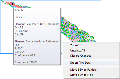
The SAE is fitting up to 72 pure elemental spectra, measured on a given SEM platform-EDS detector configuration, into a measured low-count energy-dispersive X-ray (EDX) spectrum. The SAE so called ‘element concentration’ approach then calculates the best match, by a) recording the presence of elemental spectra, and b) quantifying the relative contribution of each elemental spectra in the measured spectrum. The quality of the spectral match, as well as the measured X-ray count rate and backscatter brightness (BSE), is also recorded. The ‘elemental concentration’, or more specifically the relative contribution of elemental spectra in a measured mineral EDX spectrum, is different to the elemental mass percentage of the mineral. In the dolomite example below, the elemental weight percentages are Ca 21.7, Mg 13.2, C 13.0, and O 52.1, while ‘elemental concentrations’ are given as Ca 12.8, Mg 21.2, C 12.8, and O 23.1.

If all elements are selected for the spectra fitting operation, computing time increases. More importantly, noise is being introduced by an increasing number of partially overlapping elemental spectra. Overlapping element and element substitution rule sets are in place to limit element mismatches. If elements present in a measured spectrum have been disabled, the result would be a poor spectral match. Best results are achieved if the list of enabled elements coincides with those present in the measured sample. For O&G applications, the following 19 elements are commonly selected: C, O, Na, Mg, Al, Si, P, S, Cl, K, Ca, Ti, Cr, Mn, Fe, Cu, Zr, Ba.

Species Identification Protocol
The elemental ‘concentrations’ reported by the SAE for each individual measurement point (EDX spectrum) are compared online to the Species Identification Protocol, a list of phase definitions commonly referred to as ‘SIP list’. A measured spectrum is being assigned to a single phase, if it matches all criteria of the phase definition. Mineral phase definitions include ‘must have’ and optional ‘may have’ elemental ranges. Elemental ranges reflect the fact that multiple iterations of low-count spectra (typically 1,000 X-rays) of a single high-count spectrum necessarily results in statistical variation. In the example below, simulated low-count ranges of the high-count spectrum fit are provided for the four elements that make up dolomite: Ca 32-53, Mg 14-28, C 7-20, and O 15-32. Elemental ranges can also be used to account for natural chemical variation in a mineral. However, significant chemical variations are best approached by defining multiple end member SIP entries for a given phase. In addition to elemental ranges, elemental ratios and more complex formula can be set as rules in SIP definitions. Furthermore, optional thresholds for BSE brightness, X-ray count rate, and spectral match quality (aka ‘composition confidence’) can be defined.

In contrast to the best-match elemental fitting approach in the SAE, phase identification in the SIP is performed on a first-match basis. Phase definitions are therefore position dependent. The measured elemental concentration, BSE brightness, count rate and spectral match data of a measured spectrum is sequentially compared to all phase definitions, and mapped to the first in the SIP list that provides a match. If a measured data point does not match any predefined entry, it remains unclassified and will be reported as ‘Others’.

Expertise in SIP development is exercised by establishing elemental ranges that reliably capture all the variability inherent in low-count spectra, while preventing phase definitions to become too broad and potentially capturing spectra of non-identical phases. This expertise is often treated as valuable IP by some QEMSCAN service providers. A number of software tools are available in iDiscover, the QEMSCAN expert analysis and reporting software component, to facilitate this task. A layered approach to SIP development has previously been presented (Haberlah et al., 2011), utilising the sequential SIP approach to its full advantage. However, mineral phases characterised by large chemical variability such as some clay minerals, or mixed spectra obtained from excitation volumes that include multiple minerals, traditionally addressed as a ‘boundary phases, can remain a challenge. Boundary phases between up to four minerals can be assigned to neighbouring minerals in a statistically correct and controlled way by applying rules defined in the ‘Boundary Phase Processor’.

Primary Mineral List
Once all phases have been defined on a pixel-by-pixel basis by online SIP classification and offline application of pre-processors such as the ‘Boundary Phase Processor’, individual phases need to be grouped into real minerals or phases of interest in order to be reported as volume or weight percentage contributions. Conversion of measured phase data into chemical assays reports can be of further interest. Both are performed by grouping similar SIP phases in the ‘Primary Mineral List’ and assigning them a single density and chemical composition. In our example, dolomite would be assigned a bulk density of 2.83 g/cc and a chemical composition of weight percentages Ca 21.73, Mg 13.18, C 13.03, and O 52.06. For analysis and reporting purposes, multiple Primary Mineral List entries can further be grouped into Secondary Mineral List entries. For example, an Fe-rich version of dolomite will require a separate SIP entry for identification, and Primary Mineral List entry for adequate chemical and density characterisation. However, both dolomite entries can be grouped in the final modal mineralogy and elemental assay reports without compromising reported accuracy in composition.

The task of assigning relevant compositional data to identified phases requires a good understanding of the chemical variability inherent in some minerals comprising the sample. This task can be facilitated by including bulk compositional data from X-Ray Fluorescence (XRF) analysis. QEMSCAN software tools, such as the ‘Assay Reconciliation Report’, assist with the task of optimising chemical composition and density assumptions. Some applications in O&G are best advised to limit modal mineralogy reports to volume percentages as opposed to weight percentages, if the density values for identified phases are poorly constrained.

Sample presentation
Any discussion of automated mineralogy mineral identification and quantification would be incomplete without highlighting the impact of sample preparation and measurement setup on the results and data interpretation. Sample preparation and selected measurement area and EDX acquisition setup ultimately define reported results and how representative these are of the sample at large.

References
Haberlah, D., Owen, M., Botha, P.W.S.K., Gottlieb, P., 2011. SEM-EDS based protocol for subsurface drilling mineral identification and petrological classification, in: Broekmans, M.A.T.M. (Ed.), Proceedings of the 10th International Congress for Applied Mineralogy (ICAM), 01 05 August 2011, Trondheim, Norway. Trondheim, Norway, pp. 265–273.

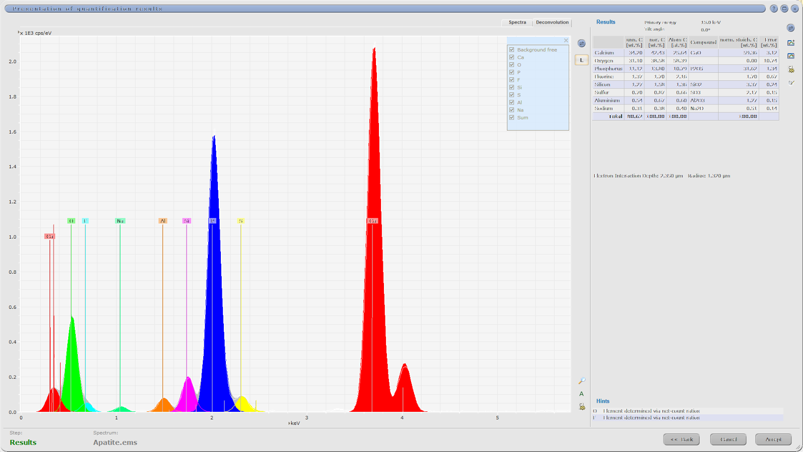
Example illustrating the fitting of elemental spectra (coloured) into a (high-count) measured dolomite spectrum (grey). The nominal elemental weight percentage of dolomite is provided, as well as the ‘concentrations’ or relative contributions of elemental spectra providing the best fit. Finally, simulated ranges for 1,000 X-rays low-count spectra are given, which would be used in the SIP entry to reliably identify the measured spectrum as dolomite.

Trace elements detection limits using QEMSCAN

In geochemistry, a trace element is a chemical element whose concentration is less than 1,000 ppm or 0.1% of a rock's composition. This definition however does not take into account the type of distribution of the element; is the element a minor and/or optional component of complex minerals (REE), and is it likely to occur as discrete mineral phases. Distribution plays a major part in how well automated mineralogy analysis can detect trace elements.

There are two different methods for QEMSCAN to detect trace elements: the first is through phase identification and calculation; the second is through direct identification in the measured energy-dispersive X-ray (EDX) spectra.

1) Trace element detection through phase identification

There are a number of requirements for trace elements to become accurately identified by mineral/phase identification:

• The phase with the trace element is intercepted in the sample surface and measured by the electron beam. Depending on the homogeneity and concentration of the phase, for this to occur will require a certain statistically defined minimum area of measurements and therefore possibly multiple cuts through the sample.
• Presence of an adequate SIP entry that correctly identifies the phase. Otherwise, it will remain 'Unclassified' (see Fig. 1).
• Presence of a phase pure enough not to result in a mixed EDX spectrum. This generally requires phases to be large enough >3-5 cubic um, depending on the accelerating e-beam voltage (15-25 kV).
• Accurate calculation of the trace element also requires that it is accounted for in the nominal or known composition of the phase, i.e. that it is a priori assigned in the Primary Mineral List and used for the elemental assay report.

2) Direct trace element detection from EDX spectrum

Similarly, for successful trace element identification from the EDX spectrum in QEMSCAN elemental maps, a number of requirements need to be fulfilled:

• The trace element must be detectable by QEMSCAN, i.e. is one of the 72 elements currently supported by the SAE (see Fig. 2).
• The element must be activated in the SIP. SIP development using the ‘element concentration method’ introduced in iDiscover 5.1 will generally try to limit the number of elements to those required to identify all typically present phases in a particular applications (e.g. 16 in the current FEI O&G SIP). The reason is that additional non-essential elements increase the background noise and thereby reduce the overall quality of mineral identification.
• The X-ray count must be adequate to discriminate the elemental energy peaks in the spectra in the elemental spectral match step of the spectral analysis. Automated mineralogy is working with low-count spectra, and depending on the application QEMSCAN is typically set to 1-5,000 X-rays per acquisition points.
• Adequate energy peak discrimination is further a function of the accelerating e-beam voltage, which, depending on the application, is set to 15-25kV. The higher the voltage, the better the resolution of the energy lines of heavier elements. However, the increase in voltage comes with an increase in the size of the excitation volume which results in more mixed spectra.
• Finally, the elemental concentration must be within the detection limits. Limited empirical tests suggest that the detection limit for lighter elements such as Mg is within 1.5-3%, REE >20%, and those in-between around 7-8%.

In conclusion, a lot depends on a priori knowledge of the sample, and the quality and relevancy of the SIP being used to measure the sample. The very fact that elemental assays are calculated in iDiscover, using assumptions on the phase composition, and that phases need to be intercepted by the measurement, arguably make X-ray_fluorescence (XRF) the preferred choice for basic reports on the chemical  bulk composition of rock samples. However, XRF cannot provide context, such as elemental deportment and textural phase association. Automated mineralogy has clear advantages over X-ray crystallography (XRD) when it comes to accurately identifying trace elements and phases - as long as they are intercepted.

Figure 1. Trace element Ti here identified in Rutile (TiO2 in red - black circles), but unidentified in Ilmenite (FeTiO3 in black - red circle)

Figure 2.  All 72 elements currently supported by elemental spectra in the new Spectral Analysis Engine (SAE) in iDiscover 5.1 (QEMSCAN)

Automated Petrography

Petrography of sectioned drill cutting as seen under optical microscope, Scanning Electron Microscope, and QEMSCAN
(the image is not part of the conference paper below) 

While compiling the 2011 publications relevant to Automated Mineralogy and Petrography for the Zotero Automated Mineralogy Library, I came across an abstract presented by Dirk van der Wal and Hans Kruseman at the VIII Congress of CIS Dressers (Ore Mining & Dressing Plants), held in Moscow during February 28 to March 2 at the at Congress Centre of the World Trade Center and organised by the Department of Enrichment of Ores NITU "MISIS", University of Moscow. This abstract presents an excellent introduction into how Automated Petrography fits into the bigger picture of Petrology and Petrograpy and is re-posted here:


Examples of Automated Petrography systems (MLA/QEMSCAN) used in the Minerals Industry

Dirk van der Wal, Hans Kruesemann
FEI Company , PO Box 80066, 5600 KA  Eindhoven, The Netherlands

Petrology is a Geoscience involved with understanding the provenance of rocks, such as depositional environment in the case of hydrocarbon reservoir rocks, or metamorphism in the case of “hard rocks”. Petrography is a branch of Petrology that involves microscopic description of mineral content and texture (microstructure) to aid interpretation of provenance.

The predominant petrographic system is a polarized optical microscope, used to identify minerals from their optical properties in crossed polarized light such as birefringes. Due to the manual and laborious nature of the technique, the Minerals Industry has struggled to deploy petrography in industrial use cases such as Geometallurgy or Mineral Processing.

Scanning Electron Microscopy (SEM) based Automated Petrography systems have been developed since the late 1980’s, predominantly in Australia (CSIRO, Univ. of Queensland), known as QEMSCAN® and Mineral Liberation Analyzer (MLA) respectively. Mineral classification technology based on backscattered electron intensity and elemental composition from energy dispersive spectroscopy has been developed over decades and provides a robust solution of automated fast mineral classification with the superior spatial resolution obtained from electron microscopy.

There are currently more than 150 Automated Petrography systems in use worldwide, predominantly in the precious and base metal mining industries. They are used to measure ore properties such as ore typing, precious metal host mineralogy, mineral associations (e.g. mineral liberation) or phase purity from core samples or grinded material.

Recent developments include advances in sample preparation and speed of analysis, aiming at reducing sample turn-around time to a point where data can be used near real-time to optimize the grinding and flotation circuit.

In this contribution, the Automated Petrography technology will be introduced and use cases illustrated from the precious metal (e.g. Pt, Au, U) and base metal mining industries (e.g. Cu, Fe).

Automated petrography applications in Quaternary Science

Cover of Quaternary Australasia Volume 28/2 December 2011 issue featuring QEMSCAN images of 2010 Brisbane Flood sediments 

While there is a strong industry focus on applying automated mineralogy and petrography analysis to petroleum exploration, mining and mineral processing, expert solutions such as QEMSCAN also provide exciting opportunities in other areas of Geoscience such as Quaternary Research. The December 2011 issue of Quaternary Australasia features a review article on "Automated petrography applications in Quaternary Science" by David Haberlah, Craig Strong, Duncan Pirrie, Gavyn K. Rollinson, Paul Gottlieb, Pieter W.S.K. Botha and Alan R. Butcher. The paper includes three compelling case studies on aeolian, fluvial and coastal sediments based on samples from the "red dawn" dust event in eastern Australia on September 23, 2009, the Icelandic Eyjafjallajökull volcanic eruptions in April 2010, the Brisbane floods in January 2011, and medieval mining impact on estuary systems along the coast of Cornwall, UK.

Abstract:
Automated petrography analysis integrates scanning electron microscopy and energy-dispersive x-ray spectroscopy (SEM-EDS) hardware with expert software to generate micron-scale compositional maps of rocks and sediments. While automated petrography solutions such as QEMSCAN® and MLA are widely used in the mining, mineral processing, and petroleum industries to characterise ore deposits and subsurface rock formations, only few Quaternary scientists have applied SEM-EDS compositional mapping to palaeo-environmental research. This paper explains the fundamentals behind the analytical method, describes the type of data that can be generated, and presents the latest advances. Potential applications in Quaternary Science are discussed, including the study of: 1) depositional and formation environments; 2) weathering and diagenetic history; 3) sediment provenancing and pathways; and, 4) the provision of complimentary data in chronostratigraphic studies. Three case studies illustrate potential applications in fluvial, aeolian and coastal research. The first case study applies automated petrography analysis to dust fingerprinting on samples collected from the ‘red dawn’ dust event that swept across eastern Australia on the 23 September 2009, and from the Icelandic Eyjafjallajökull volcanic eruptions that caused enormous disruption to air travel across Europe in April 2010. The second case study investigates flood deposits collected across Brisbane in the aftermath of the January 2011 floods. In the final case study we consider how automated petrography can aid the understanding of human impacts on the environment. Automated SEM-EDS technology was first developed by CSIRO in Australia, and made commercial by companies based in Brisbane. This proximity has proven an advantage to a wide range of researchers in Australasia pioneering innovative applications.

Reference:

Haberlah, D., C. Strong, D. Pirrie, G. K. Rollinson, P. Gottlieb, P.W.S.K. Botha, and A.R. Butcher. 2011. Automated petrography applications in Quaternary Science.Quaternary Australasia 28 (2): 3-12.

Bauxite in Southern Italy by QEMSCAN®

Researchers at the University of Napoli, Italy (Prof. Maria Boni, Giuseppina Balassone, & Nicola Mondillo), teamed up with Dr Gavyn Rollinson at the Camborne School of Mines, University of Exeter, UK, to examine bauxites from Southern Italy using QEMSCAN®. Initial results were presented at the 11th Biennial Society for Geology Applied to Mineral Deposits (SGA) Meeting held in Antofagasta, Chile, September 26-29 2011, followed up by a publication in ‘Periodico di Mineralogia’. The textural (maps) and modal data, combined with the trace mineralogy that QEMSCAN was able to offer, added an extra dimension of evidence to the study that had already used EPMA, XRD, SEM and optical microscopy techniques. Further work may be carried out to explore the issue of bauxites using QEMSCAN.

QEMSCAN® Fieldscan Image (10 mircon x-ray resolution) showing both the ooliths and matrix of a bauxite sample from Southern Italy. Field of view is 8 mm approx. It was possible to detail the variation of mineralogy in the concentric oolith rings as well as subtle differences in matrix mineralogy

References

Mondillo, N., Balassone, G., Boni, M. & Rollinson, G. 2011. Karst bauxites in the Campania Apennines (southern Italy): a new approach. Periodico di Mineralogia. 80(3).
Balassone, G., Boni, M., Mondillo, N. & Rollinson, G. 2011. Bauxite in Southern Italy: a new approach. SGA, Antofagasta, Chile. September 26th – 29th, 2011.

Environmental Mineralogy: QEMSCAN® image display

The University of Exeter, UK, has announced that it will be producing a large version of the Hayle Estuary contaminated mine waste QEMSCAN® image (produced during research at the Camborne School of Mines), to be displayed in the Library on the main campus from next spring. The image was judged with many other entries and was successfully chosen as a handful of exciting images representing research carried out at the University.

QEMSCAN WellSite launch

FEI booth at SPE ATCE 2011 launching the ruggedised, mobile QEMSCAN® WellSite™ automated petrography solution.

This has been a very exciting week and a milestone for automated mineralogy and petrography. At the Society of Petroleum Engineers' Annual Technical Conference and Exhibition (SPE ATCE 2011) in Denver, the rugged, mobile QEMSCAN® WellSite™ automated petrography solution has been launched. QEMSCAN WellSite has been developed for operation on oil and gas (O&G) drilling platforms and provides unprecedented analysis of drill cuttings. QEMSCAN WellSite has been successfully field-tested in challenging on- and off-shore drilling rig environments, in close collaboration with leading surface logging service providers and oil companies. The results of these field tests are published in the form of application notes, including this one reporting from the highlands of Papua New Guinea and conducted in collaboration with Halliburton and Oil Search Limited.

QEMSCAN WellSite is an integrated workflow solution, including sample preparation, measurement, and data analysis and export. As a result, near-real time QEMSCAN data is made available onsite, which can be used to support downhole tool data interpretation and time-critical drilling decisions.

The FEI Natural Resources website has been updated with detailed information on the QEMSCAN WellSite product, QEMSCAN WellSite technology, QEMSCAN WellSite workflow, QEMSCAN WellSite field trials, and a section on conventional and advanced mud logging. For those less familiar with petroleum exploration and production, a QEMSCAN WellSite product brochure is made available for download. Finally, for those interested in specs I recommend looking at the QEMSCAN WellSite Product Data Sheet.

QEMSCAN® elemental mapping

Colour-coded mineral and elemental QEMSCAN® maps of single dust grain collected during the 'Red Dawn' dust storm.

With iDiscover™ version 5, the new QEMSCAN® Spectral Analysis Engine (SAE) translates low-count energy-dispersive x-ray (EDX) spectra into up to 72 elemental concentrations for each measurement point. The QEMSCAN® Species Identification Protocol (SIP) assigns phase and mineral names based on elemental ranges/ratios, and optional backscatter electron (BSE) brightness thresholds, x-ray count rates, and confidence levels. An exciting new capability has been added to iDiscover version 5.2, which will officially be released in the coming week: elemental mapping.

There are likely to be many applications where elemental mapping will improve mineral identification. Here is one example, which Alan Butcher and I have developed ahead of our INQUA presentation on “SEM-EDS based particle-by-particle characterisation of a large Australian dust storm”. We presented QEMSCAN data from the massive dust storm event that swept across eastern Australia on 23 September 2009, which has been nicknamed the 'red dawn event'. As we were processing the data we asked ourselves the obvious question why don’t we see anything “red”, where are the iron oxides?

The red colour of dust is linked to sub-micron coatings of iron oxides (hematite) on mineral grains. With an excitation volume of 2-5 microns at 20 keV accelerating e-beam voltage, these coatings are too thin to be measured directly. However, they will contribute to mixed spectra. Mineral definitions generally allow for up to 5% of “other elements” to deal with matrix interference effects. Clay mineral definitions often allow for even higher iron concentrations, to account for cation exchanges. As a result, the Fe-oxide coatings did not show up in the standard SIP definitions (figure on the left). However, the Fe-oxide coatings were clearly highlighted in the Fe elemental map (centre figure). This prompted us to duplicate the quartz definition, exclude iron in the standard definition, and add an iron-rich quartz definition below. The result is shown in the figure to the right.

This simple example demonstrates three things: 1) the ability of the new QEMSCAN SAE to decompose low-count EDX spectra into elemental concentrations; 2) the ability of elemental maps to highlight the mineral context in which elements of interest occur, even in mixed spectra; 3) the beauty of position dependency of the SIP, with the first-match approach allowing to create “elemental discriminator” phase definitions.