Application of QEMSCAN in the characterisation of ultra trace PGE phases: a case study for Pt and Pd

For the high definition mineralogical study of precious metals, two methods are necessary: one method is to search, identify and quantify the precious metal mineral(s); and the second method is needed for a quantitative analysis of target element for possible refractory appearance of the target element.

Prior to the QEMSCAN and MLA era, for part one several steps would have to be taken: concentration of the heavy mineral portion of the sample, magnetic separation, and finally hand picking of the minerals of interest. Besides the time consuming and inconvenient workflow, the risk of making mistakes at each step is not negligible. Considering the very low abundances of the phases of interest, one small mistake can easily result in wrong technical conclusions!

Thanks to advances in field emission SEMs, nowadays for the first part all we need are representative aliquots in order to prepare the polished sections, the rest depends on the appropriate measurement settings to detect the trace minerals. Personally, I have detected precious metals with ppb levels in one polished section, with fairly good reconciliation with the chemical assays, that is if we are not dealing with the refractory appearance of the precious metals.

The second part - checking the invisible precious metals - is generally performed using either microprobe or laser ablation ICP-MS on handpicked target minerals, a process still necessitating long hours of hand picking under binocular microscope. In addition,we have to deal with loss of the hand-picked grains during the polishing of the section.

This case study illustrates how QEMSCAN an be applied in the detection of Pt and Pd minerals with abundances of 250-500 ppb in ultramafic rocks; and how we could skip hand picking by mapping the section and marking the target minerals for the EPMA lab.

The Project:

Four samples with elevated abundances of Pt and Pd were chosen for modal mineralogy analysis with the main objective of characterising Pt and Pd minerals/carriers. The samples are amphibolite, pyroxenite and dunite. Samples were stage pulverised to 100% passing 200 µm; 3 grams representative aliquots were split from each sample using a rotary micro plot riffler for preparing 30 mm polished sections.

The modal mineralogy analysis was performed using the default settings for BMA analysis (2.5 um pixel size) and with line space of 200 um (see Fig.1).

Fig.1. Modal mineralogy results showing major and minor minerals.

For precious metal search, we used the SMS measurement mode, while optimising the BSE threshold as well as choosing centroid X-Ray measurement for silicates. Spatial resolution was improved by using a 1 um EDS stepping interval.

With the SMS measurement mode, Pt and Pd minerals could be detected in all samples (see Fig.2). Pt is appearing as Sperrylite (PtAs2), while Pd occurs as fine native Pd grains associated with Sperrylite. Both Sperrylite and Pd appear as encapsulated grains in amphibole and quartz (see Fig.3).

Fig.2. Trace elements, the Pt minerals in each sample is less than 0.01%.

So far, we have detected and characterised the main carriers of Pt and Pd. However, the question remains whether Pt and Pd could also be present in other minerals as trace or minor elements. Regarding the mineral assembly of these samples, the only phase which can potentially accommodate Pt and Pd in their structures are Magnetite and Cr-Magnetite. In order to evaluate this, an additional quantitative elemental method like EPMA or laser ablation ICP-MS is necessary. Considering that the latter is a destructive method, we decided to proceed with EPMA.

Fig.3. Micrographs showing Pt appearing as Sperrylite (PtAs2), while Pd forms fine native Pd grains associated with Sperrylite

We selected samples 1 and 4 for additional EPMA analysis, based on the reconciliation between the Pt and Pd values between elemental assay and QEMSCAN data. Sample 1 has a large enough amount of Magnetite that proved easy to locate under the EPMA. However, this was not the case for sample 4, which has only 0.01% of magnetite. As detailed above, the conventional solution would be hand picking of the target mineral from the HMC portion of the sample under binocular microscope. The hand picked minerals were mounted in the epoxy resin, sectioned, polished and carbon coated.

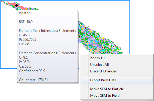
Sufficient magnetite grains could be detected by QEMSCAN in the polished section of sample 4 for EPMA analysis. However, we do not have a correlative workflow solution capable of exporting the QEMSCAN co-ordinates of these grains into the EPMA system. The alternative option is to manually look for target minerals under the EPMA, which is time consuming, especially when looking for trace minerals and therefore generally not an option when dealing with a large volume of samples. Here, we decided to make a map from the section based on the scanned fields and mark areas of interest.

We stitched the fields using the spatial mineralogy images and highlighted some of the larger particles in the centre and corners of the section, as these can be more easily located under the EPMA. Then we marked a path to the target minerals on print out maps. Our colleague at the EPMA lab could easily locate the target minerals (in this case Cr-Magnetites) using these maps which therefore allowed us to remove the problematic hand-picking step from the workflow.

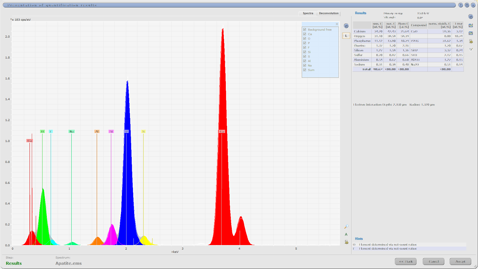
We have successfully applied this method several times to other projects involving EPMA or laser ablation analysis. We are now looking forward to developing a correlative workflow that facilitates the registration of shared coordinates. Based on the EPMA analysis, it turned out that most of the analysed Magnetites and Cr-Magnetites have up to 0.8% PtO (see Table 1).

Table 1. EPMA results from Magnetites and Cr-Magnetites. Please note that the low total of the EPMA results is because of the uncorrected values of FeO for Fe3 and Fe2.    

Summary

1. With careful sampling and sample preparation procedures in place, MLA and QEMSCAN are able to detect and characterise precious metals at trace levels as low as ppb.
2. MLA and QEMSCAN can assist in eliminating the laborious and error prone process of substituting mineral concentrate and hand picking process. However, at present the correlative workflow still requires a user to export QEMSCAN coordinates manually for subsequent EPMA or laser ablation analysis.
3. For detailed mineralogical studies, additional analytical techniques are needed to quantify elemental or isotopic compositions. In this study, the EPMA data revealed that Pt and Pd are present in the oxides as well.

Elemental quantification of phases from QEMSCAN measurements

With the recent release of iDiscover 5.3.2, a new feature has been introduced that supports the export of multiple measured EDX spectra into a single 'sum spectrum'. The QEMSCAN sum spectrum approach is quite powerful in that high-count EDX spectra can now be created over any sample selection/area of interest, with additional SIP-level control in selecting pixels of interest. This approach could be complementing the existing workflow of driving the SEM to a phase of interest located on the mineral map and collecting an online high-count spectrum on the sample. Below, the workflow of both approaches to quantifying the elemental composition of phases of interest measured in QEMSCAN data is detailed.

Targeted high-count EDX spectrum acquisition

The first approach works by selecting a field or particle of interest either in Particle View (iExplorer → Report → Particle View) or the Debug Measurements window (SIP Editor → Tools → Debug Measurements), and driving the SEM stage to the selected area. This requires the measured sample to be located within the SEM chamber, and iDiscover running on the Support PC.

In order to collect a reference spectrum on the sample, iMeasure is opened → Identify Minerals is selected in the tab, and the number of photon counts is set to something like 1,000.000, while toggling off the continuous count option. The measured spectrum can now be saved as either as an .ems or .msa file. iMeasure will need to be closed in order to open the Bruker Esprit software for elemental quantification (see below).

Combining low-count spectra into a single high-count sum EDX spectrum

The second approach is combining low-count spectra of a single or multiple phases of interest into a single high-count 'sum spectrum'. This approach can be applied to QEMSCAN data offline if the raw X-rays have been saved at the time of the measurement (Datastore Explorer → New Measurement Setup box → Field Settings → toggle on ‘Save Raw Xrays’). Sum spectra are created within the Debug Measurements window by selecting pixels, particles, fields, or samples of interest, and right-clicking → Export Pixel Data.

Step 1: Selecting the area from which particular phases are to be combined into a sum spectrum

Now, a box opens that reflects the individual and combined phases mirroring either the SIP, the Primary Mineral List, or any Secondary Mineral List selected in the above tab in ‘View using:’. In addition to combining measured spectra which have been classified into a phase by a single or multiple SIP entries, all the spectra of the selected area of interest can be combined by using a customized Secondary Mineral List that combines all phases.

Step 2: Select low-count spectra from selected area reflecting selected SIP, Primary Mineral List or Secondary Mineral List

Elemental quantification in Bruker Esprit

Quantification of the measured or exported high-count EDX spectra is performed in the Bruker Esprit software. The spectrum is opened in the Spectrum module. Elements are identified by using the Esprit Quant Tool (Quant, following selection of methodology – e.g. Interactive Oxides → Continue → Display Periodic Table → Select elements → Continue → check primary energy setting (keV) are correct → background correction (e.g. Automatic) → in options for result presentation toggle on ‘Net intensity’ (photon count without the background) → Accept. Optionally, the data can be exported into Excel (Select spectrum → Export results table).

It is advisable, to run a quality check on the number of photos making up the EDX spectrum by creating the sum of all photons in the ‘Net column’. Note that approximately a third of the photons would have been removed as background.

Step 3: Semi-quant sum spectrum. The example is based on multiple SIP definitions including boundary phase definitions for the apatite phase in the drill cutting shown above.